Bootstrap Sampling

I’m writing this post to remind myself how bootstrap sampling works. There are no proofs, only intuition, some quick experiments, and some comments.

One way to gauge the certainty of a reported result is to provide confidence estimates. This is something that bootstrap sampling can be used for, even though we only have access to a relatively small sample from the larger population of interest.

Intuition

The key idea of Bootstrap sampling is exceedlingly easy. Let’s assume that the small population to which I have access, is representative of my larger population of interest. If I repeatedly sample subsets from the small population (with replacement), and I measure a particular statistic, I can simply report the interval in which this statistic falls some fraction of the time. This becomes my confidence interval.

Let’s call the statistic \(g(.)\). Let’s assume the test population is called \(\mathcal{T} \sim \mathcal{P}\) is drawn from population \(\mathcal{P}\) In bootstrap sampling we are just simulating other possible subsets from \(\mathcal{P}\) that I could drawn, by sampling new subsets \(\mathcal{T}_i\) with replacement from \(\mathcal{T}\). My new estimate of my statistic becomes

where \(B\) is the number of simulated subsets I create. The empirical distribution of \(g\left(\mathcal{T_i}\right)\) is used to determine confidence intervals.

There is an implicit assumption here that the sampled data points are independent. In speech the use of speaker information in training systems will break this assumption if data points are individual sentences, many of which could have been spoken by the same speaker. Details about Bootstrap WER can be found here Bootstrap Confidence Intervals in ASR.

Some code is included below to illustrate how this works on a toy example. We construct \(\mathcal{T} = [t_1, t_2, \ldots, t_{100}], \ t_i \sim \mathcal{N}\left(1.3, 0.16\right)\)

Example

We construct bootstrap samples by sampling \(100\) points with replacement from \(\mathcal{T}\).

from matplotlib import pyplot as plt
import numpy as np

# Sample 100 points from gaussian mean=1.3 sig=0.4 
gauss = np.random.normal(loc=1.3, scale=0.4, size=100)

bssize_means = [] # Collect all of the bootstrap statistics     
for bs_size in range(10,20000,500):
    samples = []
    for i in range(bs_size):
        samples.append(np.random.choice(gauss, size=ssize, replace=True))
    bs_means = [np.mean(bs) for bs in samples]
    bssize_means.append(np.mean(bs_means))

An interesting question might be how many bootstrap samples are necessary for the bootstrap estimate to converge? Clearly the more bootstrap samples the better, but do we really need that many? Below is a plot of the bootstrap mean estimate as a function of the number of bootstrap samples.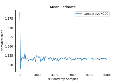

It seems only a few bootstrap samples are needed to achieve a stable estimate of the desired statistic, but if the computation is cheap, you may as well use as many as you can easily do. I’ve seen 1000-10000 recommended.

Our claim was that having small datasets would result in a lot of uncertainty about the measured statistic. In ASR, this means a small dataset causes uncertainty in model performance. So what is the relationship betweeen dataset size and the bootstrap distribution? To use the bootstrap distribution to estimate confidence intervals, it should have a large variance when the dataset is small, and a small variance when the dataset is large. Below we show the bootstrap distributions for datasets of different sizes sampled from the same population.

for s in [50, 100, 1000]:
    gauss = np.random.normal(loc=1.3, scale=0.4, size=s)
    samples = []
    for i in range(20000):
        samples.append(np.random.choice(gauss, size=s, replace=True))
    bs_means = [np.mean(bs) for bs in samples]
    plt.hist(bs_means, bins=50, alpha=0.7, label="size=" + str(s))
plt.legend()
plt.title("Bootstrap Distribution of the Empirical Mean")
plt.savefig("Bootstrap_distribution_demo.png")

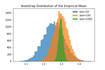
Sure enough, we find that the bootstrap distribution encodes the uncertainty we’d expect when using smaller datasets. To report a confidence interval, we can simply report the range of the middle 95% of the bootstrap simulations. Otherwise, we could model the bootstrap distribution as a Guassian or other distribution and estimate the confidence interval from the empircal variance of the bootstrap simulations.

from __future__ import print_function
print("95% Confidence interval: (", np.percentile(bs_means, 2.5), ", ", np.percentile(bs_means, 97.5), ")")

In our case the 95% confidence interval for the 1000 sample dataset was \((1.27195901268, 1.32081083565)\).

Bootstrap Confidence Interval in Kaldi

For anyone using Kaldi, the bootstrap confidence interval is computed by default using the script ./steps/score_kaldi.sh or the binary compute-wer-bootci. After running most of the kaldi examples you can find the relevant file in exp/MODEL_NAME/decode_DATASET/scoring_kaldi/wer_details/wer_bootci.

That’s about it.