Lattice Free Maximum Mutual Information (LF-MMI)
- 14 minsI’m writing this to remember all of the details of MMI and LF-MMI, especially the gradient computation that I worked through with Desh Raj. I probably missed a few things, but hopefully the main concepts are covered. If you are reading this and you already know what MMI is and you are just looking for the details of LF-MMI, skip to the LF-MMI section. I added some very basic information about ASR with HMMs just for the sake of completeness. The original paper is here.
tldr;
LF-MMI is just like lattice based MMI, but replaces utterance specific denomiator lattices with a globally shared denominator graph constructed by means of a 4-gram phone language model. Some tricks to prevent overfitting are usually required including cross-entropy regularization via multitask learning and L-2 regularization on the network outputs. Since the network is directly trained to produce pseudo-likelihoods, no prior normalization is required.
The LF-MMI objective function is a particular discriminative objective function used especially in hybrid HMM-DNN ASR. Discriminative objective functions are of interest because they allow us not only to train models to make the correct output sequence more likely, but they also learn to make incorrect sequences less likely. In other words they are trained to maximize the separation between the correct and incorrect answers, or to discriminate between correct and incorrect answers rather than simply assign high weights to the correct sequences.
One such objective function is called the Maximum Mutual Information (MMI) objective function. It is also sometimes referred to as Maximum Conditional Likelihood Estimation. LF-MMI is essentially just the MMI objective function that has been modified to enable training ASR systems on GPU. I describe these modificaitons later. For now, I am just going to describe the MMI objective function.
Relationship of Maximum Mutual Information Objective to Mutual Information
The MMI objective function is called MMI, because it can be derived from maximizing the mutual information between the input \(X\), and output \(W\) sequences. First the MMI objective function is defined to be
\[F_{MMI} = \sum_{r=1}^N \log{\frac{p_{\theta}\left(X_r | W_r\right)p\left(W_r\right)}{\sum_{W} p_{\theta}\left(X_r | W\right)p\left(W\right)}}\]In this function, \(r\) indexes the training examples (utterances or short chunks of audio), \(X_r\) are the audio features corresponding to chunk \(r\), and \(W_r\) is the reference transcript. Probability density functions (PDFs) subscripted by \(\theta\) are those parameterized with learnable parameters \(\theta\). This objective function can be shown to be equivalent to maximizing the mutual information over the parameter space between the input and output sequences.
\[arg\max_\theta I_\theta \left(X_r; W_r\right) = arg\max_\theta H\left(W_r\right) - H_\theta\left(W_r | X_r\right)\]In general since we are only trying to model the relationship between inputs and outputs, the only parameters we are able to optimize are those responsible for the conditional distribution \(p_\theta\left(W | X\right)\). The distribution \(p\left(W\right)\) is estimated from the training transcripts and is considered fixed. In the case of ASR, this simply corresponds to a language model.
From this we see that the above optimization problem is equivalent to
\[arg\max_\theta H\left(W_r\right) - H_\theta\left(W_r | X_r\right) = arg\min_\theta H_{\theta}\left(W_r | X_r\right)\]Using the definition of conditional entropy we have that
\[\begin{align} \mbox{ (1) } H_{\theta}\left(W_r | X_r\right) &=& E_{p\left(X_r, W_r\right)} \left[ - \log{p_{\theta}\left(W_r | X_r\right)}\right] \\\ \mbox{ (2) } &=& E_{p\left(X_r, W_r\right)} \left[ - \log{\frac{p_{\theta}\left(X_r | W_r\right) p\left(W_r\right)}{p\left(X_r\right)}}\right] \\\ \mbox{ (3) } &=& E_{p\left(X_r, W_r\right)} \left[ - \log{\frac{p_{\theta}\left(X_r | W_r\right) p\left(W_r\right)}{\sum_{W} p_{\theta}\left(X_r | W\right) p\left(W\right)}}\right] \end{align}\]Line (1) from above is the from the definition of conditional entropy. Line (2) uses Bayes rule to factorize the posterior distribution. Line (4) simply factorizes the joint distribution \(p_{\theta}\left(X, W\right)\) into a product of the conditional and marginal distributions.
Then, using the law of large numbers we note that …
\[E_{p\left(X_r, W_r\right)} \left[ - \log{\frac{p_{\theta}\left(X_r | W_r\right) p\left(W_r\right)}{\sum_{W} p_{\theta}\left(X_r | W\right) p\left(W\right)}}\right] = \lim_{N \to \infty} \frac{-1}{N} \sum_{r=1}^N\log{\frac{p_{\theta}\left(X_r | W_r\right) p\left(W_r\right)}{\sum_{W} p_{\theta}\left(X_r | W\right) p\left(W\right)}}\]So finally, by approximating this limit by using a finite sample size \(N\) …
\[E_{p\left(X_r, W_r\right)} \left[ - \log{\frac{p_{\theta}\left(X_r | W_r\right) p\left(W_r\right)}{\sum_{W} p_{\theta}\left(X_r | W\right) p\left(W\right)}}\right] \simeq \frac{-1}{N} \sum_{r=1}^{N}\log{\frac{p_{\theta}\left(X_r | W_r\right) p\left(W_r\right)}{\sum_{W} p_{\theta}\left(X_r | W\right) p\left(W\right)}}\]And we convert the minimization problem
\[arg\min_{\theta} H_{\theta}\left(W_r | X_r\right)\]into a maximization problem by negating the conditional entropy and dropping the constant \(N\) which is just a scaling factor and won’t change the optimal parameter values. This leaves us with the originally presented expression for the MMI objective function.
Acoustic Modeling with HMMs Background
The HMM acoustic model is constructed as follows.
- Words are modeled as a sequence of units. In traditional ASR these units are triphones, but even just a sequence of letters would probably work fine. A single word could corresponding to different allowable sequences of units.
EITHER –> IY - TH - ER
EITHER –> AY - TH - ER
- For each of these units, there is an associated HMM. Traditionally this is a 3-state HMM, but for reasons I’ll explain later, we tend to use a 1-state HMM instead. It would look something like this …
.png)
- In an HMM we model \(p_{\theta}\left(X_r | W_r\right)\) where \(X_r = \{x_0, \ldots, x_{T-1} \}\) is a length \(T\) sequence as …
\(\pi_r\) corresponds to one of the valid paths through the HMM for the word sequence \(w_r\). \(\pi_r^t\) is the state at time \(t\) along the path \(\pi_r\).
Gradient of MMI
I am going to assume that the underlying acoustic model is an HMM. I assume we are using a Hybrid HMM-DNN model, where the DNN output activations are used as log emission probabilities for the \(D\) states \(s_1, \ldots, s_D\) in our HMM. We define \(y_s^t\) to be the DNN activations at time \(t\) for a state \(s\). In other terms \(y_s^t = \log{p_{\theta}\left(x_t | s \right)}\)
We also note that since the transition probabilities are not trained, we will just consider these to be a multiplicative weight associated with a particular path (i.e. \(K_{\pi_r} = \prod_{t=0}^{T-1} p\left(\pi_r^t | \pi_r^{t-1}\right)\)).
Plugging this into the expression for \(F_{MMI}\) and converting the logarithm of a product into the sum of the logartihms we get
\[\begin{align} F_{MMI} &= \sum_{r} \log{\frac{p\left(w_r\right) \sum_{\pi_r}K_{\pi_r} e^{\sum_{t=0}^{T-1}y_{\pi_r^t}^t}}{\sum_{w} p\left(w\right) \sum_{\pi_w}K_{\pi_w} e^{\sum_{t=0}^{T-1}y_{\pi_w^t}^t}}} \\\ &= \sum_{r} \left[ \log{p\left(w_r\right)} + \log{\sum_{\pi_r}K_{\pi_r} e^{\sum_{t=0}^{T-1}y_{\pi_r^t}^t}} - \log{\sum_{w, \pi_w} p\left(w\right) K_{\pi_w} e^{\sum_{t=0}^{T-1}y_{\pi_w^t}^t}} \right] \end{align}\]Now since we are modeling the emission probabilities using a neural network trained using backpropagation and automatic differentiation, we really only need the partial gradient with respect to the output activations of the neural network \(y_s^t\).
\[\begin{align} \frac{\partial F_{MMI}}{\partial y_s^{\tau}} &= \frac{\partial}{\partial y_s^{\tau}} \sum_{r} \left[ \log{p\left(w_r\right)} + \log{\sum_{\pi_r}K_{\pi_r} e^{\sum_{t=0}^{T-1}y_{\pi_r^t}^t}} - \log{\sum_{w, \pi_w} p\left(w\right) K_{\pi_w} e^{\sum_{t=0}^{T-1}y_{\pi_w^t}^t}} \right] \\\ &= \sum_{r} \frac{\partial}{\partial y_s^{\tau}} \left[ \log{p\left(w_r\right)} + \log{\sum_{\pi_r}K_{\pi_r} e^{\sum_{t=0}^{T-1}y_{\pi_r^t}^t}} - \log{\sum_{w, \pi_w} p\left(w\right) K_{\pi_w} e^{\sum_{t=0}^{T-1}y_{\pi_w^t}^t}} \right] \\\ &= \sum_{r} \frac{\partial}{\partial y_s^{\tau}} \left[\log{\sum_{\pi_r}K_{\pi_r} e^{\sum_{t=0}^{T-1}y_{\pi_r^t}^t}} - \log{\sum_{w, \pi_w} p\left(w\right) K_{\pi_w} e^{\sum_{t=0}^{T-1}y_{\pi_w^t}^t}} \right] \\\ &= \sum_{r} \left[ \frac{\partial}{\partial y_s^{\tau}} \log{\sum_{\pi_r}K_{\pi_r} e^{\sum_{t=0}^{T-1}y_{\pi_r^t}^t}} - \frac{\partial}{\partial y_s^{\tau}} \log{\sum_{w, \pi_w} p\left(w\right) K_{\pi_w} e^{\sum_{t=0}^{T-1}y_{\pi_w^t}^t}} \right] \\\ &= \sum_{r} \left[ \frac{1}{\sum_{\pi_r}K_{\pi_r} e^{\sum_{t=0}^{T-1}y_{\pi_r^t}^t}} \cdot \frac{\partial}{\partial y_s^{\tau}} \sum_{\pi_r}K_{\pi_r} e^{\sum_{t=0}^{T-1}y_{\pi_r^t}^t} - \frac{1}{\sum_{w, \pi_w} p\left(w\right) K_{\pi_w} e^{\sum_{t=0}^{T-1}y_{\pi_w^t}^t}} \cdot \frac{\partial}{\partial y_s^{\tau}} \sum_{w, \pi_w} p\left(w\right) K_{\pi_w} e^{\sum_{t=0}^{T-1}y_{\pi_w^t}^t} \right] \\\ &= \sum_{r} \left[ \frac{1}{\sum_{\pi_r}K_{\pi_r} e^{\sum_{t=0}^{T-1}y_{\pi_r^t}^t}} \cdot \sum_{\pi_r}K_{\pi_r} \frac{\partial}{\partial y_s^{\tau}} e^{\sum_{t=0}^{T-1}y_{\pi_r^t}^t} - \frac{1}{\sum_{w, \pi_w} p\left(w\right) K_{\pi_w} e^{\sum_{t=0}^{T-1}y_{\pi_w^t}^t}} \cdot \sum_{w, \pi_w} p\left(w\right) K_{\pi_w} \frac{\partial}{\partial y_s^{\tau}} e^{\sum_{t=0}^{T-1}y_{\pi_w^t}^t} \right] \\\ &= \sum_{r} \left[ \frac{1}{\sum_{\pi_r}K_{\pi_r} e^{\sum_{t=0}^{T-1}y_{\pi_r^t}^t}} \cdot \sum_{\pi_r}K_{\pi_r} e^{\sum_{t=0}^{T-1}y_{\pi_r}^t} \frac{\partial}{\partial_s^{\tau}} \sum_{t=0}^{T-1}y_{\pi_r^t}^t - \frac{1}{\sum_{w, \pi_w} p\left(w\right) K_{\pi_w} e^{\sum_{t=0}^{T-1}y_{\pi_w^t}^t}} \cdot \sum_{w, \pi_w} p\left(w\right) K_{\pi_w} e^{\sum_{t=0}^{T-1}y_{\pi_w^t}^t} \frac{\partial}{\partial y_s^{\tau}} \sum_{t=0}^{T-1}y_{\pi_w^t}^t \right] \\\ &= \sum_{r} \left[ \frac{1}{\sum_{\pi_r}K_{\pi_r} e^{\sum_{t=0}^{T-1}y_{\pi_r^t}^t}} \cdot \sum_{\pi_r}K_{\pi_r} e^{\sum_{t=0}^{T-1}y_{\pi_r^t}^t} \mathbb{1}\left(\pi_r^\tau, s\right) - \frac{1}{\sum_{w, \pi_w} p\left(w\right) K_{\pi_w} e^{\sum_{t=0}^{T-1}y_{\pi_w^t}^t}} \cdot \sum_{w, \pi_w} p\left(w\right) K_{\pi_w} e^{\sum_{t=0}^{T-1}y_{\pi_w^t}^t} \mathbb{1}\left(\pi_r^\tau, s\right)\right] \end{align}\]Here we introduced the indicator function
\[\begin{align} \mathbb{1}\left(\pi_r^\tau, s\right) = \begin{cases} 1 & \pi_r^\tau = s \\\ 0 & \pi_r^\tau \neq s \end{cases} \end{align}\]We are almost done now. We note that the numerator of the first term in our expression corresponds to the joint probability of the acoustic sequence \(X_r\) going through any path for which \(\pi_r^{\tau} = s\). Note that we have restricted the set of paths to be those that correspond to the word sequence \(W_r\). Using the forward and backward probabilities at each time step we can write this as \(p\left(X_r, \pi_r^\tau = s\right) = \alpha_r\left(s, \tau\right) \beta_r\left(s, \tau\right)\). In the denominator we can partition the set of paths into the set of all paths that use a state \(s\) at time \(\tau\). In this way when we sum over all of the states at time \(\tau\) we are in fact summing over all paths. Hence we can rewrite the denominator as \(\sum_{\sigma} \alpha_r\left(\sigma, \tau \right) \beta_r\left(\sigma, \tau\right)\).
The second term in our expression can be decomposed in the same way as the first term. The only difference is that the set of paths is now the set of paths that are valid for any possible word sequence. We can still represent this as an HMM where paths for different word sequences are weighted by the probability of those word sequences. The state space just happens to be much larger. We will name the forward and backward probabilities associated with the space of all possible words \(\alpha_{w^\ast}\left(s, \tau\right), \beta_{w^\ast}\left(s, \tau\right)\).
Our expression for the gradient then becomes …
\[\begin{align} \frac{\partial F_{MMI}}{\partial y_s^{\tau}} &= \sum_{r} \left[ \frac{\alpha_r\left(s, \tau\right) \beta_r\left(s, \tau\right)}{\sum_{\sigma} \alpha_{r}\left(\sigma,\tau\right) \beta_{r}\left(\sigma, \tau\right)} - \frac{\alpha_{w^\ast}\left(s,\tau\right) \beta_{w^\ast}\left(s, \tau\right)}{\sum_{\sigma^\prime} \alpha_{w^\ast}\left(\sigma^\prime,\tau\right) \beta_{w^\ast}\left(\sigma^\prime, \tau\right)}\right] \\\ &= \sum_{r} \left[ \gamma_{r}\left(s, \tau\right) - \gamma_{w^\ast}\left(s, \tau\right)\right] \end{align}\]Algorithm
We now almost have an algorithm for computing the gradient with respect to a neural network output!
-
Create a graph (HMM) representing the space of all possible word sequences. To do this you could imagine enumerating all possbile word sequences. You could then enumerate all possible pronunciations of each word sequences. Finally you would chain together the HMM models for the phonemes present in each of these pronunciations. Taking the union of all such HMM chains would correspond to the graph of all possible word sequences. We call this the denomiator graph as it corresponds to the denominator in the MMI objective function.
-
For each audio chunk \(X_r\), create a graph that corresponds to the reference word sequence. This corresponds to the union of all HMM chains that correspond to the ground truth word sequence for the audio chunk \(X_r\). We call this the numerator graph as it corresponds to the numerator in the MMI objective function.
-
Use the DNN to produce outputs \(y_s^t\) for the audio chunk \(X_r\).
-
Using these outputs, run the forward and backward algorithm on both the numerator and denominator graph to generate \(\alpha_{r}\left(s, t\right), \beta_{r}\left(s, t\right), \alpha_{w^{\ast}}\left(s, t\right), \beta_{w^\ast}\left(s, t\right)\)
-
Compute the gradient according to
where \(\theta\) is some parameter in the neural network, and that gradient is just computed via autograd and backpropagation.
Our algorithm has some major problems, however, especially the way we proposed to generate the numerator and denominator graphs. Below are details explaining how in practice we can generate these graphs. The main contribution of LF-MMI is how it approximates this graph in order to make the computation feasible and the graph of a manageable size. In practice this is all done using Finite State Transducers (FSTs), which enable us to compactly store the set of all possible sequences needed in (1.) for instance. I will be making another post about FSTs in ASR, specifically on the decoding graph and the components used to create it in a future post HCLG.
LF-MMI
In order to make the denominator graph a manageable size, the following modifications are made to the denominator graph:
-
The denominator graph uses a 4-gram phone language model instead of a word level language model. The space of phones is much smaller than the space of all words. Furthermore, the language model is not smoothed; smoothing introduces many back-off states and edges which increases the size of the denominator graph.
-
The HMM topology used is the one state topology described above (as opposed to the 3-state topology). Again this makes the denominator graph smaller, and speeds up the forward / backward computation.
-
The DNN output frame rate is also reduced from 1 frame/10ms to 1 frame/30ms for the same reasons.
Training with chunks
In order to train on chunks that are smaller than a whole utterance, there are a number of other necessary changes as well.
- The utterance level HMMs are represented as finite state transducers (FSTs). A separate FST acceptor is constructed that enforces a chunk of audio to be roughly aligned with the single best state sequence. The FST is created by having 1 node per time step. Between each node are a set of edges representing the set of state-ids that are allowable at this time step. This set is constructed from looking at a user specified window around the single best path and allowing any of the pdfids in this window to be accepted at the specific time. By composing this FST with the utterance level HMM, we get back a lattice representing the set of all probable alignments of the audio to the HMM states. Alternate paths in the resulting lattice therefore correspond to alternative pronunciations or alternative alignments of the audio. In this way, each state in the lattice is associated with a particular time index, which allows us to chop the utterance level lattices into chunks. Note that since we use state-tied parameters for HMMs in ASR, we actually align to pdf-ids (which could be shared across state), rather than on state id.
The time enforcer FST looks like the FST shown below. For more information on the time enforcement, read Improving LF-MMI Using Unconstrained Supervisions for ASR, which is where the image below comes from.
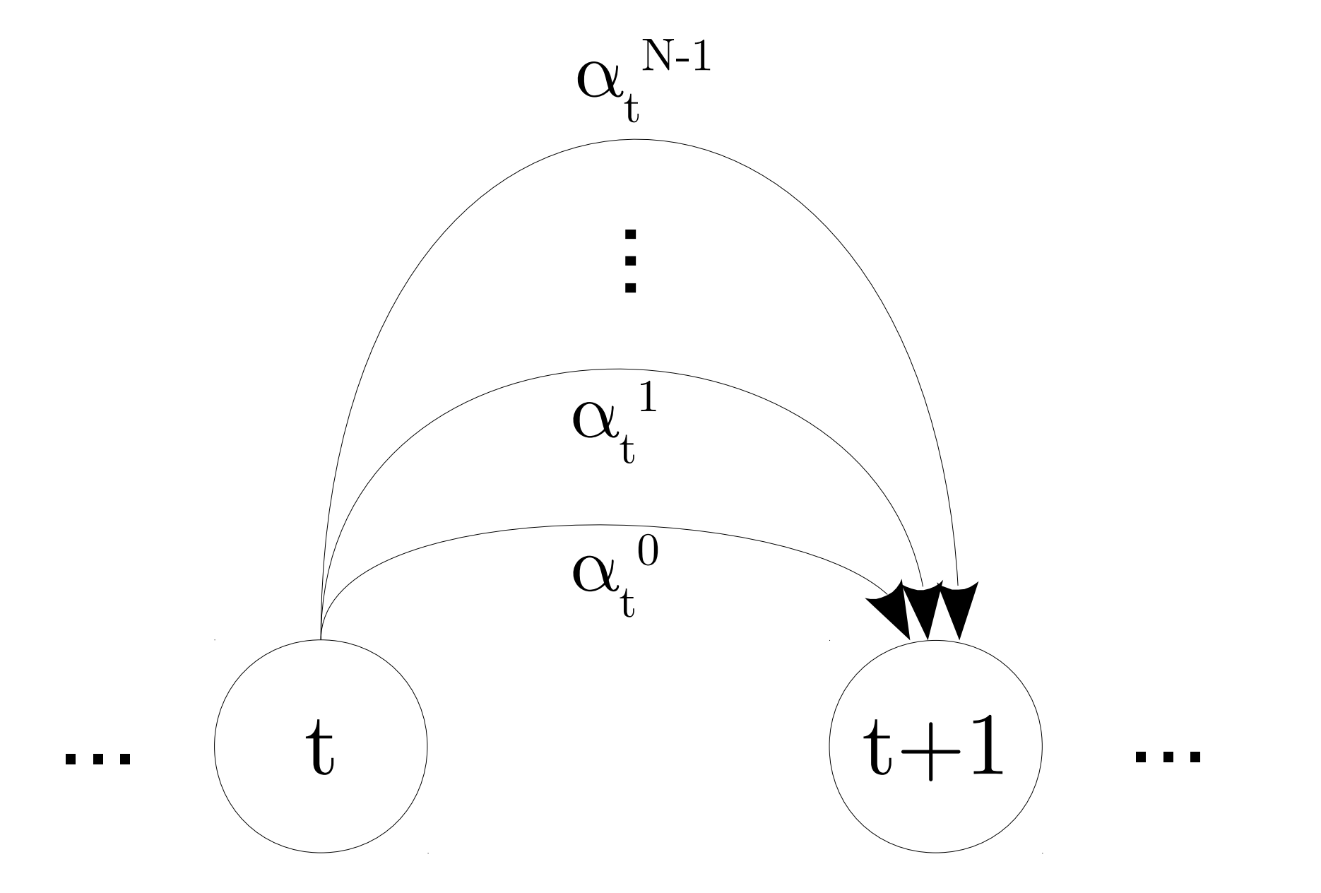
where \(\{\alpha_t^k | k \in \left[0, N-1\right]\}\) is the set of \(N\) distinct pdf-ids allowed at time \(t\).
-
The denominator graph is created using a language model trained on full utterances. Since we are using chunks of audio, this means we could be both starting and ending in the middle of an utterance. Clearly, the initial and final probabilities of the initial denominator graph would be wrong if that were the case. To compensate for this we use modified initial and final probabilities. The final probability at every state is set to 1. This lets the utterance end at any arbitrary HMM state (not just at the end of the utterance). New initial probabilities are computed by creating the first 100 steps of the FST trellis. The state occupancy probabilities are averaged across all 100 time steps. We use this average as our new initial probabilities for each state. This modified denominator graph is called the normalization fst.
-
Finally, since the numerator and denominator graphs are created in different ways, we need to ensure that the set of paths in the numerator graph is a subset of those in the denominator graph. We do this by composing the numerator graph with the normalization fst. To avoid double counting the transition probabilities, they are actually omitted in the original numerator graph.
Regularization
The LF-MMI objective was observed to overfit. 3 methods of regularizing the network are used to prevent overfitting.
-
Multitask training with the cross-entropy objective. The forward probabilities at each time step in the numerator graph are used as soft targets instead of the usual hard targets.
-
L-2 regularization on the network outputs. In otherwords, the network is trained using the objective. \(F_{LF-MMI} = F_{MMI} + \lambda {\left\lVert y^t\right\rVert}_2^2 + \omega F_{xent}\)
-
A Leaky HMM is used. Here a small transition probability between any two states is allowed. This allows for gradual forgetting of context.